Mobile robotics in simulation with ROS 2 - Part 1: The lab
Introduction
I studied Robotics, and my last robotics project was in ROS 1: a robot that drove to a goal while avoiding obstacles with a LiDAR, reading ArUco markers along the way. Since then my work has moved toward ML. Now, with ROS 2, this project brings the two worlds together.
The series builds a mobile robot (camera, 2D lidar and gyro) layer by layer, in a room full of ArUco markers:
| Part | Topic |
|---|---|
| 1 | The lab |
| 2 | Perception: markers and the current pose |
| 3 | Safety: LiDAR |
| 4 | Spatial awareness: where am I? |
| 5 | Fusion: odometry, gyro and markers |
| 6 | Adaptation: applied machine learning |
The question behind this first part is a concrete one: how do I know that what the robot believes is true? A robot never sees the world directly. It infers it from what its sensors report. Before building anything on top of that, I need a way to compare what it infers with what actually happened.
Why do it in simulation, and not physically from day one?
Simulation may not be realistic, and every chapter will say so. One of the biggest challenges in robotics today is getting what works in simulation to work in the real world: real physics brings disturbances, measurement errors and changes in the environment nobody planned for. Even so, simulation lets this series get its first results the right way: by repeating, measuring with statistics and comparing alternatives.
The first part sets up the lab: the world, the reference everything gets measured against, and the robot.
The chosen architecture
The lab has three pieces:
- Gazebo. It simulates the room and the robot. Since it computes the world's physics, it knows exactly where everything is at every moment.
- The robot's software. It has no access to that information about the world. It only gets what its sensors give it (the camera image, the lidar distances, the gyro's turn rate and how far each wheel turned) and works out from there where it is, just as a real robot would.
- The experiment. It gets both: what the robot computes and believes, and what really happened in the generated world. Its job is to compare the two measurements.
The world
It's an 8 x 8 m room with ten ArUco markers (15 cm per side), placed in spots that are hard for the camera to reach:
| Id | Where | Case it covers |
|---|---|---|
| 0 | on a post facing the robot | near and head-on |
| 1, 2 | on posts turned 30° and 60° | seen from the side |
| 3 | on the floor | flat, below the camera |
| 4 | on the side of a box | out of the starting view |
| 5 | on the far wall | far away |
| 6, 8 | on walls, high and tilted down | above the camera |
| 7, 9 | on the side walls and the back wall | the robot has to turn to see them |
A fiducial marker is easy to read head-on and up close. A robot rarely gets that view: it sees markers far away, at an angle, on the floor or above the camera.
The world lives in build_world.py, where each marker is described by where it sits and which way it faces:
PLACEMENTS = [
    Placement(0, (0.5, 0.0, 0.6), _turned_from_robot(0.5, 0.0, 0), "post", "facing the robot"),
    Placement(1, (1.5, 1.3, 0.7), _turned_from_robot(1.5, 1.3, 30), "post", "turned 30 degrees"),
    Placement(3, (0.2, -0.5, 0.001), (0, 0, 1), "floor", "on the floor"),
    # ...
]
One modelling detail mirrors the real object: a printed marker can only be read from the front, and in the simulation the image goes on just one face of the panel. If it could be read from behind, the robot would place itself on the wrong side of the marker.
This is how the robot's camera sees the room from its start pose (top) and turned 37° toward the box (bottom). Green marks the markers the detector managed to read, with the distance it measures, and amber the ones in view that it didn't read:
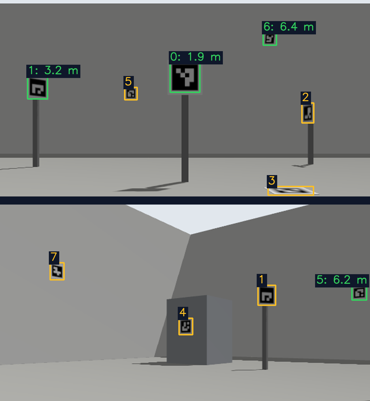
At the top, six markers are in view and the detector reads three. At the bottom, the large marker on the nearby post (1) and the one on the box (4) are clearly visible and go unread, while a tiny one about 5.5 m away (5) gets read. Why that happens is the question for Part 2.
Decision 1: what is the robot's belief compared against?
To know whether the robot is right, I need a reference. There are three candidates:
| Option | What it compares | Why it falls short, or why it works |
|---|---|---|
| Watching it in RViz | what the robot computed | there is nothing to compare it against, and it stays as that "result" |
| Trusting the command | "I asked for two turns, it did two turns" | the command may be what did not happen: the wheels can slip and the motor can be slow to respond |
| Gazebo's true pose | the exact pose Gazebo's physics computes | only exists in simulation, and a physical robot will face disturbances |
This is how it's done outside simulation too. In labs, the answer comes from motion capture systems: cameras around the room that track reflective markers attached to the robot, with millimetre precision. Well-known odometry and localization benchmarks are built this way. That level of precision comes at a very high price. In simulation it comes for free, and simulating first is one of the best practices in robotics.
So what Gazebo measures goes out on a channel of its own that no node of the robot has access to. It works like the answer key to an exam: if the student (the robot) could see it, the exam would stop measuring anything.
To use it, every experiment follows the same steps: put the robot in a known situation, give it a command, record what the robot believes and what actually happened, and repeat under several conditions. A second script turns those records into tables and plots.
Main character: the robot
The robot in this series is generic on purpose: a 36 x 24 cm base with two driven wheels and two sliding supports, a forward-facing camera 25 cm off the floor, a 360° 2D lidar on a mast, and a gyro.
Decision 2: how is it described?
Describing the robot starts with the fact that each of its parts has its own point of view. The camera sees a marker "2 m in front of me", the robot needs to know it's "2 m in front of my centre", and the map needs it "at this point in the room". In ROS, the system that translates between those points of view is called TF, and each point of view is a reference frame:
The robot is described once, in a URDF file. This tree comes from it, and so does the robot Gazebo simulates. With two separate descriptions, moving the camera 2 cm in one could shift every detection by those 2 cm without anyone noticing.
Gazebo's true pose stays out of this tree. If it were in it, any node could look it up.
Decision 3: how fast can it change speed?
A real motor needs time to brake and to accelerate. Gazebo lets you set those limits, but its configuration has a catch: if you only set the maximum speeds and accelerations, braking becomes instant. That's why the robot sets every limit in both directions, which also covers braking, reversing and turning right.
Decision 4: how does the wheel touch the floor?
To estimate how far it has moved, the robot counts how far each wheel has turned. That estimate is called odometry.
To turn in place, the robot drives one wheel forward and the other backward. How much it turns depends on how far apart the wheels push against the floor: the closer together they push, the more it turns for the same wheel motion. The odometry assumes each wheel pushes from its centre.
In the simulation, each wheel needs a contact shape: whatever actually touches the floor. There are two natural options:
- Flat contact: the wheel touches the floor with the same shape it's drawn with, a cylinder. The simulator rests that cylinder on its edges, and when turning it pushes from the inner ones, which are closer together than the odometry assumes.
- Point contact: what touches the floor is a sphere the size of the wheel. It touches at a single point right under the centre, exactly where the odometry assumes.
To decide, I ran a simulation test: two full turns in place, comparing how far the robot believes it turned with how far it really did. I repeated it at three speeds, in both directions, three times each.
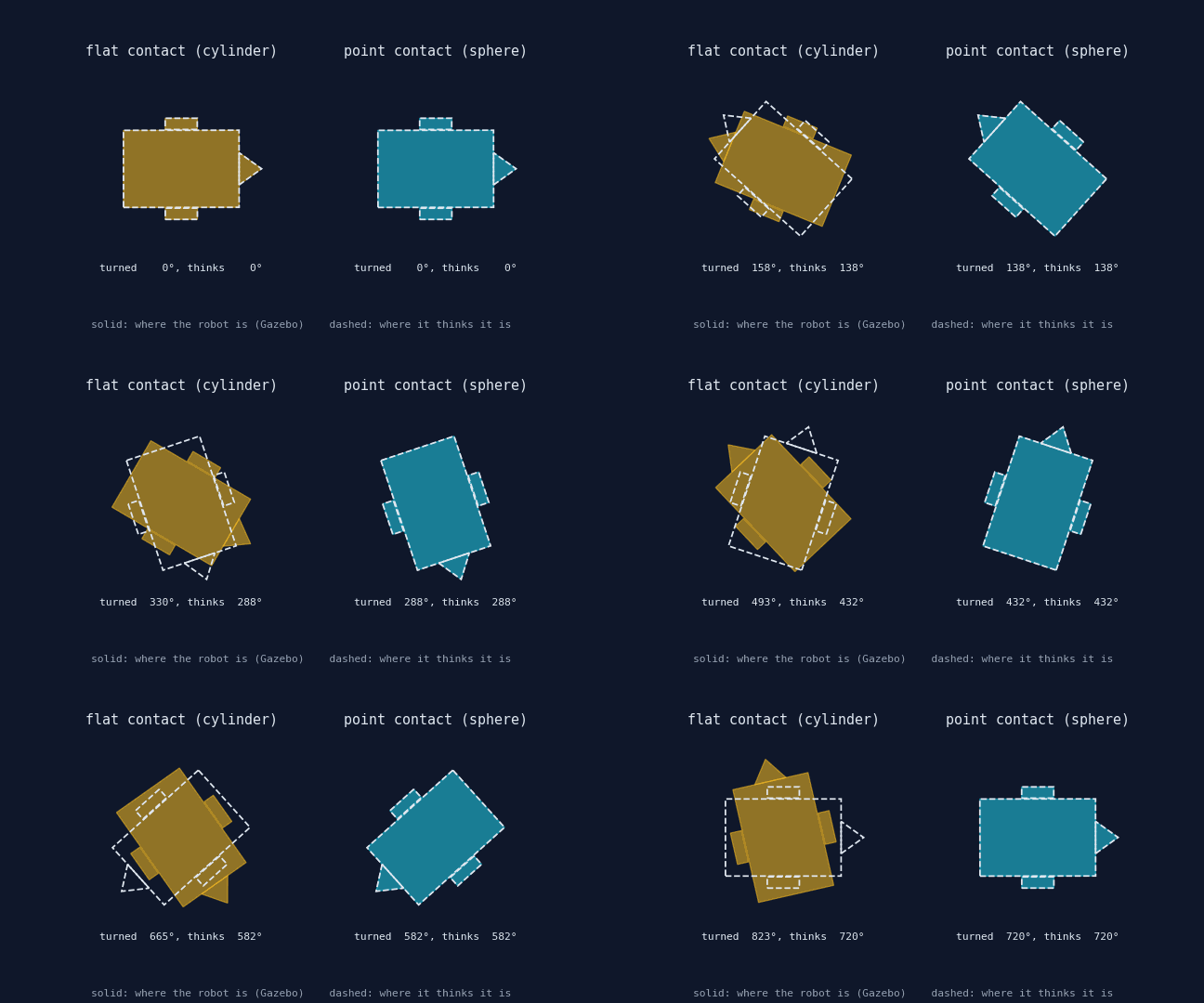
| Contact | What the odometry reports, as a share of the true turn |
|---|---|
| Flat (cylinder) | 87.5% |
| Point (sphere) | 100% |
With flat contact, the robot turns roughly 14% more than it believes: by the end of the two turns, the gap between where it is and where it thinks it is comes to about 100°. The robot uses point contact. On a flat floor, its wheels then behave like thin real wheels that touch the floor right under their centre.
Limitations
- Clean images and fixed lighting. No sensor noise, no motion blur and no lens distortion. This only measures the best case.
- The sphere is only a contact model. On a flat floor (like this world's) it behaves like a thin wheel, but on a slope or a step it would behave like a ball rolling under gravity.
- Gazebo's odometry is exact apart from the physics: it comes from each wheel's rotation, without the noise of a real encoder.
- Gazebo is deterministic: the same commands give the same numbers every time, without the random variation of the real world.
- This isn't the final test. Nothing measured here replaces testing on a real robot. It gets us to that test with the method already validated.
Wrapping up
The lab is ready: the world is generated and the robot is connected to ROS 2. From here on, what the robot believes can be measured statistically against what actually happened.
Coming up in Part 2
Perception: how a ROS 2 node detects the markers live, how their position relative to the camera is worked out, and how far off that position gets with distance and angle.
The full code can be found at github.com/KevDP/ros2-aruco-world. To regenerate this part's numbers:
experiments/sim.sh wheel_collision:=sphere -- python3 experiments/turning.py --label sphere
experiments/sim.sh wheel_collision:=cylinder -- python3 experiments/turning.py --label cylinder
python3 experiments/turning_report.py
experiments/sim.sh -- python3 experiments/camera_views.py --stock