Mobile robotics in simulation with ROS 2 - Part 5: Fusion
Introduction
Part 4 left the robot knowing where it is whenever it sees a marker closer than 4 m. Between one marker and the next it has nothing of the kind, and on this part's route that is most of the time. The wheels and the gyro do measure how the robot moves at every moment, though each goes wrong in its own way, and this part brings the three sources together.
The subject is:
- How each source goes wrong.
- How two filters bring them together.
- How far from its true position the robot ends up along a route.
The question behind this part is: how well does the robot know where it is along a route, whether it sees markers or not?
The chosen architecture
Both filters are ekf_node nodes from robot_localization, the ROS 2 implementation of an extended Kalman filter. A filter like this predicts where the robot moved from what it knows of its motion and corrects that prediction with every measurement, weighing each source by its covariance. The wheel odometry arrives with its drift from noisy_odometry, the gyro goes through gyro_calibration first, and the fixes come from Part 4's localizer.
The sources
| Source | What it measures | How it goes wrong |
|---|---|---|
| Wheels | how far the robot moved and turned | a small error at every step, which adds up without limit |
| Gyro | how fast it turns | a little noise, and a bias that changes every time it starts |
| Fixes | where it is in the room | it only updates when it detects a marker closer than 4 m, a few centimetres off |
The wheels and the gyro tell how the robot moved since the last instant, and the fixes tell where it is.
Decision 1: one filter or two?
| Option | What it means |
|---|---|
| A single filter with everything | whenever a fix arrives, it can swing between smooth motion and a large jump |
| Only wheels and gyro | smooth, but the error can grow without limit |
| Two filters | one gives a smooth pose that drifts over time, and the other corrects it with the fixes |
ROS defines a mobile robot's frames: map, odom and base_footprint. ekf_local combines wheels and gyro and publishes odom -> base_footprint, which never jumps. ekf_global adds the fixes and publishes map -> odom, the drift corrected so far, which does jump when a fix arrives. A controller reads odom and moves without jolts, and whatever needs the robot's place in the room reads map.
Decision 2: what does the filter take from the wheels and the gyro?
| Option | What it means |
|---|---|
| The pose each sensor integrates | the filter swings between the two poses |
| The orientation Gazebo gives | it is the true heading, and in the real world this would not work the same way |
| The speeds: the wheels' forward speed and turn rate, the gyro's turn rate | the filter integrates once, and each speed is weighed by its covariance |
From the wheels, the filter also takes a sideways speed of zero, since a robot in differential drive cannot move sideways.
Decision 3: what to do with the gyro's bias?
A low-cost gyro has a small bias. The covariance the gyro publishes describes only its noise, and when the robot turns, this error goes into the heading and pushes the estimate off course with every metre the robot drives.
| Option | What it means |
|---|---|
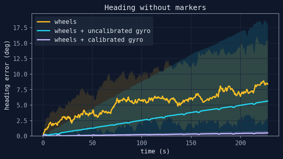
| Use the gyro as it comes | the heading error grows with time (6° at the end of the route, median) |
| Use only the wheels | the wheels' turn is further off, with 8° in the median |
| Calibrate at power-up, while at rest | 0.5° in the median, in exchange for the robot waiting still for a few seconds at power-up |
gyro_calibration averages the gyro for 5 s with the robot still and subtracts that average from every reading. If the robot moves during those seconds, it starts over. This method is used by the well-known TurtleBot3, which calibrates its gyro at power-up.
Decision 4: how far should each reading be trusted?
Every time the camera reads a marker whose place is on the map, the localizer works out where the robot has to be to see the marker that way. That result (x, y and heading) is a fix.
Each fix comes with its covariance, which is how far off it can be. It is drawn as an ellipse that grows with distance (an uncertainty ellipse), and grows faster sideways than along the line of sight.
Fixes from one view arrive about 15 times a second with nearly the same error, and the filter adds each one up as if it were new. If that view is off, the filter ends up where the view says. At start-up, for instance, the robot stands still at its true pose, and as soon as the first fixes arrive the filter moves 9 cm.
The filter also has a gate: it drops a fix that lies more than a set number of sigmas from what it expects, counting its own uncertainty and the fix's. A sigma is one standard deviation of that combined uncertainty. For example, if the filter expects the robot with 10 cm of combined uncertainty, a fix that lands 40 cm away sits at 4 sigmas, gets through a 5σ gate and is dropped by a 3σ one. These are the options, with the median of the 30 runs and the worst of them:
| Option | Mean error along the route | Largest error | Largest error in the worst run |
|---|---|---|---|
| 5σ gate | 12.6 cm | 33 cm | 5.9 m |
| 3σ gate | 12.3 cm | 31 cm | 47 cm |
| 5σ, every fix's covariance ×4 | 11.5 cm | 30 cm | 5.9 m |
| 5σ, covariance ×16 | 10.4 cm | 28 cm | 5.8 m |
| 5σ, only 2 fixes a second | 9.9 cm | 30 cm | 6.7 m |
A larger covariance, or fewer fixes to correct the filter, makes the combined uncertainty larger, and a far fix then sits at fewer sigmas and gets through the gate more easily. As the table shows, with the 3σ gate no run went past an error of 1% of the route's length, and that is why it stays.
Fixes arrive late
A fix comes from an image that went through the detector and the localizer, and it reaches the filter 29 ms after the image was taken (median). The global filter keeps a second of history and applies each fix at its image's instant, and the delay does not turn into position error.
The result
To measure it, an experiment repeats the same route 30 times:
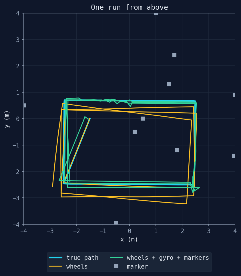
- Three laps of a 5 × 3.2 m rectangle around the room, 51 m in about 4 minutes.
- Gazebo's true pose steers the robot, and every run follows the same path.
- Each run starts a new simulation, with its own wheel drift and its own gyro bias.
A marker was in view 22% of the time.
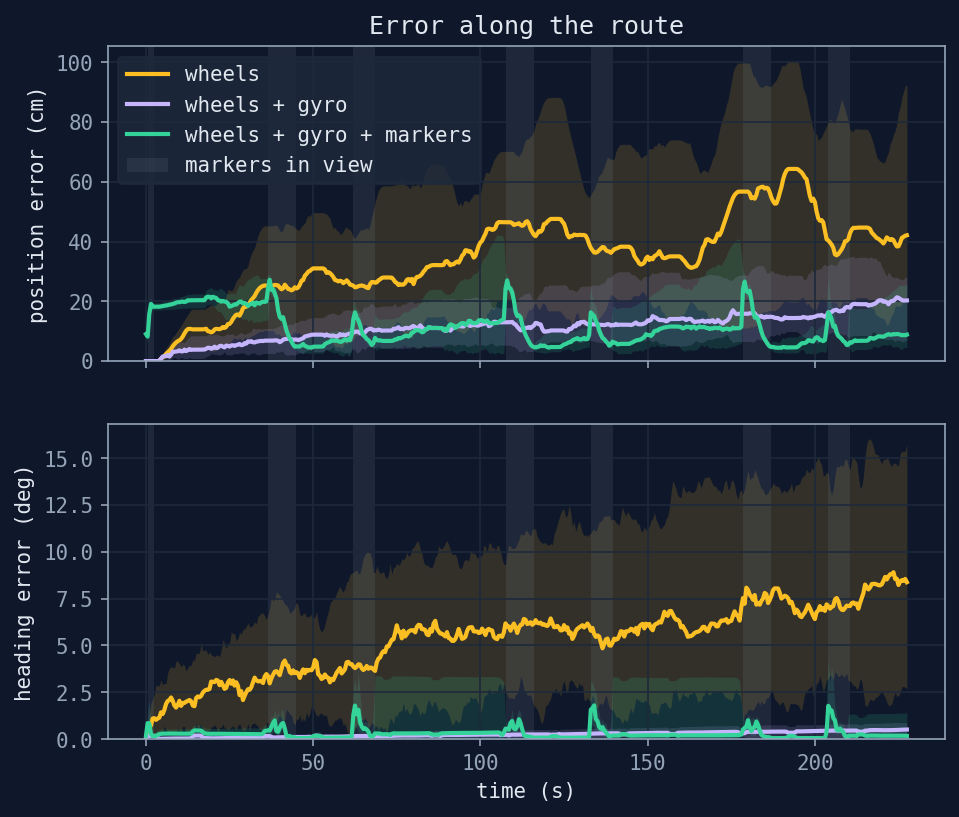
With the median of the 30 runs:
| Estimate | Mean error | End of lap 1 | Lap 2 | Lap 3 | Heading at the end |
|---|---|---|---|---|---|
| Wheels | 36 cm | 32 cm | 35 cm | 41 cm | 8.4° |
| Wheels and gyro | 11 cm | 11 cm | 14 cm | 20 cm | 0.5° |
| Wheels, gyro and markers | 12 cm | 11 cm | 11 cm | 9 cm | 0.2° |
- The wheels alone drift further and further, above all in heading.
- With the calibrated gyro the heading barely moves, and the error grows slowly.
- With the markers the error does not grow from one lap to the next. Averaged over the route it is close to the wheels and gyro, because the fixes bring their own error, but that error does not add up.
Limitations
- The bias is measured once. A real gyro's bias also changes with temperature and time, and this calibration does not follow it. The robot also has to stay still for a few seconds after it starts.
- The noise generated for the wheels is only random. A real robot's also has a part that always pulls the same way.
- The route is driven with the true pose. No controller uses the estimate yet, and its errors do not change the robot's path.
Wrapping up
The robot now knows where it is along a route, whether it sees markers or not. With the calibrated gyro and the markers it ends each lap about 9 to 11 cm from the true position, and the error does not grow. The wheels alone end up 41 cm off. It remains to measure how much each fix can be trusted, and Part 6 takes it on.
Coming up in Part 6
Learning: the robot keeps its own fixes as data, labels them itself and learns to recognize the mirrored ones in each new place.
The full code can be found at github.com/KevDP/ros2-aruco-world. To regenerate this part's numbers:
for run in $(seq 1 30); do
  experiments/sim.sh detector:=true drift_seed:=$run -- python3 experiments/fusion.py --run $run
done
python3 experiments/fusion_report.py